L. Buono, A. D'Amore, G. Giuliani, F. Polonara
Dipartimento di Energetica, Università di Ancona
60100 Ancona, Italia

Introduction

The rapid freezing of food stuffs is a process that simultaneously guarantees a better product quality and a greater productivity for the food industry. An important factor to ensure rapid freezing is to work with very low temperatures of the refrigerant fluid: the use of liquid nitrogen in such applications (normal boiling temperature -196°C) is a classic, but it carries the drawback that using a fluid at nearly -200°C to cool a product to -18°C is an obvious thermodynamic absurdity. The same efficacy as liquid nitrogen, in terms of freezing rate, can be obtained by using the refrigerant fluid at temperatures of around -75°C: given that, in the majority of applications, the final vehicle for transferring the heat energy to the product is air, the option of the reversed Joule-Brayton cycle, in which the working fluid is air, is of considerable interest.
With this in mind, a research project coordinated by TecnoMarche (the scientific and technological park of the Marche region in Italy) was organized with a view to designing, implementing and testing a system for freezing ready-to-eat foods comprising a revolving drum freezer operating with air at -75°C produced by a refrigerator operating on an air cycle.
This paper describes the prototypes of freezer chamber and refrigerator that have just been constructed and the simulation techniques used to optimize the freezing process.

Prototype of refrigerator operating on an air cycle

The reversed gas, or Joule-Brayton cycle has been used extensively in the past for refrigeration applications wherever the fundamental requirements included the compact dimensions of the equipment (for instance, for air conditioning on board aircraft). This system is far less efficient than the steam compression cycle, however, and this fact prevents its genuinely widespread use.
The loss of efficiency with the reversed gas cycle by comparison with the steam compression cycle diminishes progressively, however, with lower temperatures of the cold source, as shown in the analysis in Figure 1.

Figure 1 - Trend of the efficiency of different types of reversed cycle
(hot source temperature =30°C, vapour compression cycles: DT exchangers =10 K, efficiency of the air cycle: first-stage compressor =0.80,
second-stage compressor =0.75, turbine=0.82)

The refrigerator, made using Japanese technology (AIRS, Kajima Corp.), operates on a reversed Joule-Brayton double-compression air cycle with intermediate inter-refrigeration and internal regeneration.
The two compression stages are implemented by two centrifugal compressors, the second of which is coupled mechanically to the turbine acting as an expansion organ. The compressor-turbine assembly (bootstrap) is made using European technology (Atlas-Copco).
Internal regeneration is achieved with an exchanger using a secondary fluid (silicone oil) that enables an end-of-expansion temperature of -75°C to be achieved.
The refrigeration cycle is interrupted as necessary by a defrosting cycle, in which the regeneration cycle and the freezer are disabled, while the turbine is bypassed.
The machine comprises the following main components (Figure 2):
­ first-stage compressor
­ first inter-refrigeration exchanger (water cooled)
­ second-stage compressor
­ second inter-refrigeration exchanger (water cooled)
­ intermediate-fluid heat regenerator (high-pressure side)
­ turbine
­ ice trap
­ drum freezer (external user)
­ intermediate-fluid heat regenerator (low-pressure side)

Figure 2 - Block diagram of the AIRS machine operating on an air cycle

The compressor is a classic centrifugal compressor driven by an electric motor operating at a voltage of 200 Vac, controlled by an inverter with a frequency variable from 50 to 60 Hz and connected to an overgear so that its rotation can be varied from 30,000 to 36,000 rpm. The various operating stages enable the temperature of -75°C to be reached gradually.
Once it has been compressed, the hot air is sent to the first heat exchanger (a finned coil), where it undergoes the first cooling phase by means of water coming from a dedicated circuit.
From the first exchanger, the air goes to the second compressor, subsequently passing into a second heat exchanger, which is also a finned coil connected to the same cooling circuit as the first exchanger.
The temperature of the air is further lowered before it is sent to the turbine, passing through an intermediate-fluid heat regenerator (high-pressure side).
Once it has left the turbine, and before it is sent to the freezer, the air is diverted through a snow trap, which intercepts any frost forming in the part of the circuit at a temperature of less than 0°C; the presence of the snow trap makes it necessary to provide for a defrosting cycle at high temperatures so that the build-up of ice can be eliminated fairly quickly.
The air is subsequently sent to the external user through a dedicated circuit. On leaving the user, before it is sent back to the compressor, the air passes through the regenerator again (low-pressure side).
As mentioned earlier, the first and second heat exchangers are served by the same cooling circuit, composed of a recirculating pump on the warm side and one on the cold side, a plate exchanger and a chiller. The operation of all the various elements involved (pumps and fans) is governed by the AIRS control system.
In the case of the present installation, logistic problems made us decide not to use the chiller, thus also excluding the pump on the cold side and using the water in the circuit at the industrial plant where the prototype is installed as the cooling fluid instead.
The intermediate-fluid heat regenerator is composed of two finned batteries served by a closed circuit comprising a tank containing the intermediate fluid, which is a silicone oil (given the low temperatures required). The silicone oil is circulated by means of a suitable pump in the high-pressure regenerator, where it removes heat from the air in order to restore said heat to the air in the regenerator on the low-pressure side.

Prototype of revolving drum freezer

The freezer is composed of central circular body, shaped rather like a drum, that contains the products to freeze; a flow of cold air is delivered to the drum from the refrigerator. The air exchanges heat with the products and is discharged through a pipe lying coaxial to the delivery pipe (Tout=-60°C)
Figure 3 shows a picture of the freezer prototype, with the opening for loading and unloading the food products at the front, and the delivery and return air pipes at the back.

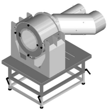
Figure 3 - Prototype of revolving drum freezer

The freezer is coupled to an electric motor that enables a rotating movement of the drum, at a speed that can vary continuously between 6 and 30 rpm, so as to prevent the food products from sticking to the inside walls.

Modeling methods used to optimize the freezing process

The aim of fluid thermodynamic analysis, implemented in this case using CFD (Computational Fluid Dynamics) techniques, is to obtain a detailed analysis of the heat exchange between the products and the cold air so as to be able to take action by means of geometrical modifications to the delivery and/or return piping in the event of any problems of uneven freezing of the products. It is also important to estimate the time it takes to freeze the product.
After the fluid thermodynamic analysis, the mathematical model will be validated by means of a series of measurements at the test bench, using thermocouples and a hot wire anemometer for point-by-point temperature and velocity measurements in order to assess any differences with respect to the results obtained with the calculation procedure.
The fluid thermodynamic analysis was carried out by simplifying the problem. First of all, a two-dimensional problem of the freezer was considered, disregarding the relative motion; then we analyzed the case in which the machine was made to turn at a constant speed; and, finally, the problem was dealt with from a three-dimensional point of view.
The sequence of steps involved in studying a problem with computational fluid dynamics is listed below:
­ analyzing the problem in question in detail, with a view to simplifying the case considered in the study;
­ constructing the calculation mesh;
­ establishing the thermophysical properties of the materials involved;
­ establishing the initial and boundary conditions;
­ analyzing the results obtained (temperatures, velocities, pressures, etc.).
First of all, a mesh was created with 9000 cells, represented in Figure 4.
An implicit segregated, non-stationary model was prepared as the solution-finder.
Moreover, the energy equation was enabled and the following were assumed as the boundary conditions:
­ INLET: the inlet conditions of the fluid were specified, i.e. temperature (Tin = -75°C), density (variable with temperature, according to the ideal gas equation), velocity ((vin= 8 m/s), turbulence conditions (intensity of turbulence equating to 10% and turbulent mixing length amounting to 0.02 m).
­ OUTLET: no particular outlet conditions were specified because the simulation program proceeds directly with the calculation of the various parameters.
The conditions of the WALL were also defined, considering that the walls must be conductive: the program calls for a separation of the solid and fluid cells by means of a wall when the heat transmission is enabled.
The decision to study the two-dimensional case initially was dictated mainly by the calculation times needed by the program's solution-finder. The number of cells used to schematically represent the calculation domain was also chosen with the calculation times in mind. To give an idea, we can say that the calculation time needed for the two-dimensional model is of the order of several hours, whereas for three-dimensional models, with the number of cells amounting to around 500,000, the calculation takes several days (and we have to remember that said times are dead times in the design phase and must consequently be reduced as far as possible).

Figure 4 - Calculation mesh

After these essential introductory considerations, we can go on to provide an overview of the preliminary results obtained so far, relating to the velocity and temperature profiles, since the greatest constraint lies in relation to the variation in temperature between the freezer inlet and outlet.
The figures given below show examples of the temperatures and velocities in the calculation mesh, without adding any food products, in order to analyze the thermal flows exchanged between the freezer and the outside environment first.
The transient case is illustrated (i.e. also simulating the rotation of the drum), which is more realistic in the case in point. You can follow the evolution of the flow through the freezer from an initial instant up until such time as a thermal equilibrium is achieved. From then on, we can assume that the analysis is complete and verify the results obtained.
Figures 5 and 6 compare the velocity vectors in the calculation mesh at two different times.
Figure 5 represents the velocity vectors at the time t=0.002 s: in practical terms, we obtained an image of the moment when the first cold flow arrives in the freezer and the velocity vectors separate out symmetrically, then leave through the return pipe.
In Figure 6, at the time t=1.9 s, the flow has transited through the freezer to depart through the return pipe. A common feature of the cases represented in the two figures is the reflux of the fluid, which deviates as soon as it enters the freezer in order to leave through the return pipe. This phenomenon was confirmed by the fact that the velocity of the fluid tends to diminish progressively as it comes closer to the freezer's cover. While, on the one hand, the reflux of cold air represents a hazard for the successful outcome of the product freezing process, on the other it represents a positive factor for the air cycle, which requires a fluid return at a temperature no higher than approximately -60°C.

Figure 5 - Velocity vectors at time t=0.002 s

Figure 6 - Velocity vectors at time t=1.9 s

Figures 7 and 8 show the temperature profiles at two different times.

Figure 7 - Temperature profile at time t=0.002 s

Figure 8 - Temperature profile at time t=1.9 s

In Figure 7 the cold front advances slowly through the freezer and tends to separate, confirming the reflux phenomenon already encountered with the velocity vectors.
Figure 8 shows the temperature distribution at the time t=1.88 s. The return temperature averages around -70°C, while the temperature inside the freezer, even in the most "critical" areas, never exceeds -44°C.

Conclusions

The next steps in our research will be oriented towards establishing potential fluid thermodynamic variations inside the freezer as a result of changes to the geometry of the refrigerated air intake pipe.
Then various products will be placed on the floor of the freezer to assess the heat load absorbed and the feasibility of freezing the product with an I.Q.F. (Individually Quick Frozen) type of treatment.